[논문 리뷰] High-Resolution Image Synthesis with Latent Diffusion Models(Stable Diffusion)
arXiv 2021. [Paper] [Github]
Robin Rombach, Andreas Blattmann, Dominik Lorenz, Patrick Esser, Björn Ommer
Ludwig Maximilian University of Munich & IWR, Heidelberg University, Germany | Runway ML
20 Dec 2021
1. Introduction
이미지 합성은 Computer vision에서 최근에 많은 발전을 이룬 분야이다. likelihood 기반의 모델들과 Autoregressive(AR) transformers, GAN 등의 모델이 사용되었다. 최근에는 Diffusion model이 이미지 합성 분야에서 인상적인 성능을 보였으며, 특히 class-conditional 이미지 합성과 super-resolution에서는 SOTA를 달성하였다.
Democratizing High-resolution Image Synthesis
Diffusion Model은 likelihood기반 모델로 mode-covering으로 인해 세부 정보를 모델링하려고 하기 때문에 computing cost가 크다. DDPM의 reweighted 목적함수는 초기 노이즈 제거 단계에서 적게 샘플링해서 이 문제를 해결하려하지만 모델을 학습, 평가하려면 RGB 이미지의 고차원 공간에서 반복적인 gradient 계산이 필요하기 때문에 여전히 computation cost가 크다. Diffusionmodel에 대한 접근성을 높이고 컴퓨팅 리소스를 줄이려면 학습 및 샘플링에 대한 computation demands를 줄이는 것이 핵심이다.
Departure to Latent Space
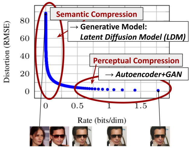
픽셀 공간에서 이미 학습된 Diffusion model에 대한 분석으로 시작한다. 위 그림은 학습된 모델의 rate-distortion trade-off를 보여준다.
- rate-distortion: 특정 수준의 품질을 유지하면서 이미지에서 압축할 수 있는 정보의 양을 측정하는 것. Diffusion model에서 rate-distortion은 high-frequency details(perceptual compression)과 데이터의 의미론적 및 개념적 구성 학습(semantic compression) 간의 균형을 평가하는데 사용된다.
다른 likelihood 기반 모델과 마찬가지로 학습은 두 단계로 나눌 수 있다.
- Perceptual compression: high-frequency detail들을 제거하지만 의미(semantic)은 거의 학습하지 않는 단계
- Semantic compression: 실제 생성 모델이 의미론적(semantic) 구성과 개념적(conceptual) 구성을 학습하는 단계
저자들은 먼저 perceptual하게 동등하지만, 계산적으로 더 적합한 공간을 찾는 것을 목표로 하며 고해상도 이미지 합성을 위해 Diffusion model을 합성시킨다. 저자들은 학습 과정을 두가지 단계로 나누었다.
- 데이터 space와 perceptual하게 동일한 저차원 representation space로 보내는 autoencoder를 학습한다. 이전 연구와는 다르게 잠재 공간에서 Diffusion model을 학습시키기 때문에 과도한 space 압축에 의존하지 않아도 된다.
- 네트워크를 한 번만 통과해 latent space에서 효율적인 이미지 생성이 가능하다. 이 모델을 LDM(Latent Diffusion Models) 라고 한다.
이 접근 방식의 주목할만한 점은 보편적인 autoencoding 단계를 한번만 학습하고, multi Diffusion model 학습을 위해서는 재사용도 가능하고 완전히 다른 task를 탐색할 수 있다는 것이다. 이를 통해 다양한 image-to-image, text-to-image task를 위한 여러가지 Diffusion model을 효율적으로 탐색할 수 있다.
Contributions
- 순수한 transformes 기반 모델과 다르게 본 논문의 모델은 더 높은 차원으로 확장된다.
- 계산 비용을 낮추고 unconditional image synthesis, inpainting, stochastic super-resolution 와 같은 task와 데이터셋에서 계산 비용을 절감했다.
- encoder/decoder 아키텍처와 score 기반 연구를 동시에 학습하는 이전 연구와 다르게 본 연구는 reconstruct, generate 능력의 섬세한 가중치를 요구하지 않는다.
3. Method
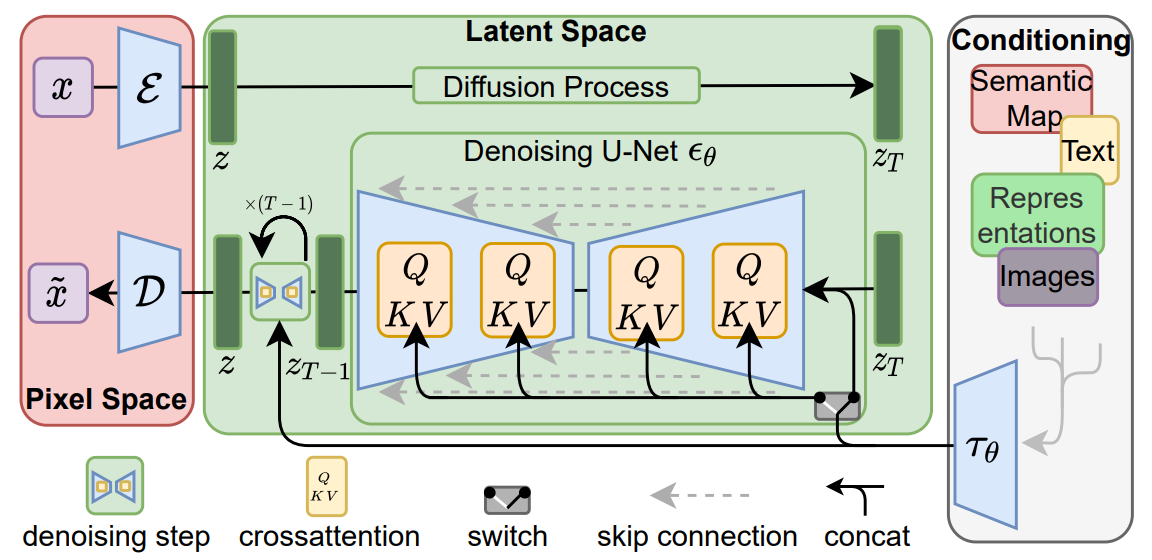
고해상도 이미지 합성에 대한 Diffusion model 학습의 계산량을 줄이기 위해 Diffusion model이 해당 loss term을 적게 샘플링해서 perceptual하게 관련 없는 detail들은 무시할 수 있지만, 픽셀 space에서 계산 비용이 많이든다. 저자들은 학습 단계에서 압축을 명시적으로 분리해 이러한 단점을 보완한다 (Fig2 참고). 이를 위해 이미지 space와 perceptual 하게 동일한 공간을 학습하지만 계산 복잡성을 줄이는 autoencoding 모델을 활용한다. 이러한 접근법의 장점은 다음과 같다.
- 고차원 이미지 space를 남겨두고 저차원 space에서 샘플링이 수행되기 때문에 계산적으로 효율적이다.
- Unet 아키텍처에서 상속된 Diffusion model의 inductive bias를 활용하여 공간 구조가 있는 데이터에 효율적이다.
- Latent space가 여러 생성 모델을 훈련하는데 사용될 수 있고 downstream task(CLIP-guided synthesis)에도 활용 가능한 general-purpose 모델을 얻는다.
3.1 Perceptual Image Compression
저자들의 Perceptual compression 모델은 이전 연구들을 기반으로 perceptual loss와 patch-based adversarial objective의 조합으로 학습되는 autoencoder로 구성된다. 이것은 local realism이 적용되어 reconstruction이 이미지 manifold에 국한되고 $L_2$ 또는 $L_1$ objective 와 같은 pixel space loss에만 의존해 발생하는 bluriness를 방지할 수 있다.
$x \in \mathbb{R}^{H \times W \times 3}$의 이미지가 RGB space에 주어지면, encoder $\mathcal{E}$가 $x$를 latent representation $z=\mathcal{E}(x)$로 인코딩하고, 디코더 $\mathcal{D}$가 latent $z \in \mathbb{R}^{h \times w \times c}
$로부터 이미지를 재구성하여 $\tilde{x} = \mathcal{D}(z) = \mathcal{D}(\mathcal{E}(x))$를 만든다. 인코더는 이미지를 factor $f = H/h = W/w $로 downsample하고 $m \in \mathbb{N}$에 대해 factor를 $f = 2^m$으로 둔다.
latent space의 분산이 커지는 것을 피하기 위해 저자들은 두 가지 다른 regularization로 실험하였다.
- $KL-reg$ : VAE와 유사하게 학습된 latent에서 표준 정규분포에 대해 약간의 KL-penalty를 부과한다.
- $VQ-reg$ : 디코더 내에서 vector quantization layer를 사용한다. 이 모델은 VQGAN으로 해석될 수 있지만 quantization layer가 디코더에 의해 흡수된다.
LDM은 학습된 latent space $z=\mathcal{E}(x)$의 2차원 구조와 작동하도록 만들어져 상대적으로 약한 compression을 사용하고 좋은 reconstruction을 만들 수 있다. LDM의 compression 모델은 $x$ detail을 더 잘 보존한다. (Tab.8 참고)
$\rightarrow$ 이전의 $z$의 임의의 1차원 순서에 따라 분포를 autoregressive하게 모델링하여 $z$의 고유 구조를 무시한 모델링과 대조된다. 3.2 Latent Diffusion Models
Diffusion Models
Diffusion model은 정규분포를 길이가 $T$로 고정된 Markov chain의 reverse process(denoising) 과정을 거쳐 $p(x)$ 분포를 학습하도록 설계된 모델이다. 이미지 합성에서 가장 성공적인 모델들([Guided Diffusion Models][DDPM][SR3])은 denoising score matching을 미러링하는 $p(x)$에 대한 variational lower bound를 reweighted한 변형을 사용한다. 이러한 모델은 입력 $x_t$의 noise가 제거된 변형을 예측하도록 학습된 denoising autoencoder $\epsilon_\theta (x_t, t) (t = 1, \cdots, T)$의 동등하게 가중된 시퀀스로 해석할 수 있다. 해당 목적식은 다음과 같이 단순화 할 수 있다.
$$L_{DM} = \mathbb{E}_{x, \epsilon \sim \mathcal{N} (0,1), t} \bigg[ | \epsilon - \epsilon_\theta (x_t, t) |_2^2 \bigg]$$
Generative Modeling of Latent Representations
$\mathcal{E}, \mathcal{D}$로 구성된 perceptual compression 모델을 사용해 Generative Modeling of Latent Representations , 저자들은 high-frequency를 감지할 수 없는 detail이 추상화 되는 효율적이고 낮은 차원의 latent space에 접근할 수 있었다. 고차원의 픽셀 space와 비교해, 이 latent space는 2가지 이유로 likelihood 기반 생성 모델에 적합한다.
- 데이터의 중요한 semantic bit에 집중할 수 있다.
- 더 낮은 차원에서 학습하고, 계산적으로 훨씬 효율적이다. high-compression된 autoregressive, attention 기반의 transformers와 같은 이전 연구와 다르게 LDM 은 이미지별 inductive bias 를 활용할 수 있다.
- inductive bias:2D convolutional layer들로 UNet을 구성하는 것이 포함되고 아래와 같이 reweighted bound를 사용하여 perceptual하게 가장 관련성이 높은 비트에 목적식을 집중시키는 것도 포함된다.
$$L_{LDM} := \mathbb{E}_{\mathcal{E}(x), \epsilon \sim \mathcal{N}(0,1), t} \bigg[ | \epsilon - \epsilon_\theta (z_t, t) |_2^2 \bigg]$$
neural backbone $\epsilon_\theta (\cdot, t)$는 time-conditional UNet으로 구현된다. Forward process는 고정된 상태로 학습 중에 $z_t$를 $\mathcal{E}$에서 효율적으로 얻을 수 있고 $p(z)$의 샘플을 $\mathcal{D}$에 한 번 통과시켜 이미지 space로 디코딩할 수 있다.
3.3 Conditioning Mechanisms
Diffusion models은 $p(z|y)$ 형식의 조건부 분포를 모델링할 수 있다. 조건부 denoising autoencoder $\epsilon_\theta(z_t,t,y)$로 구현되며, 입력 $y$를 통해 text, semantic map, image-to-image 변환과 같은 합성 프로세스를 조정할 수 있다.
저자들은 cross-attention 매커니즘을 UNet backbone에 보강해 diffusion model을 유연한 image generator로 만든다. 다양한 종류의 $y$를 전처리하기 위해 $y$를 중간 representation으로 만드는 $\tau_\epsilon (y) \in \mathbb{R}^{M \times d_\tau}$ 도메인 특화 encoder $\tau_\theta$를 사용한다. 그런 다음 cross-attention layer를 통해 UNet의 중간 lyer에 맵핑된다.
$$\textrm{Attention}(Q, K, V) = \textrm{softmax}(\frac{QK^T}{\sqrt{d}}) \cdot V
Q = W_Q^{(i)} \cdot \phi_i (z_t), \quad K = W_K^{(i)} \cdot \tau_\theta (y), \quad V = W_V^{(i)} \cdot \tau_\epsilon (y)$$
$\phi_i (z_t) \in \mathbb{R}^{N \times d_\epsilon^i}$는 $\epsilon_\theta$를 구현하는 UNet의 중간 representation이며, $W_Q^{(i)} \in \mathbb{R}^{d \times d_\tau}$, $W_Q^{(i)} \in \mathbb{R}^{d \times d_\tau}$, $W_K^{(i)} \in \mathbb{R}^{d \times d_\tau}$는 학습 가능한 projection matrices이다.
이미지, condition 쌍을 기반으로 아래 식을 통해 conditional LDM 을 학습한다.
$$L_{LDM} := \mathbb{E}_{\mathcal{E} (x), y, \epsilon \sim \mathcal{N} (0, 1), t} \bigg[ | \epsilon - \epsilon_\theta (z_t, t, \tau_\theta (y)) |_2^2 \bigg]$$
$\tau_\theta$와 $\epsilon_\theta$는 위 식으로 동시에 최적화된다. 각 도메인별 기존 모델에 의해 $\tau_\theta$가 파라미터화할 수 있기 때문에 conditioning 매커니즘은 유연하다고 할 수 있다.